
Excel CHOOSE Function
The Excel CHOOSE function returns a value from a given data range or array based on the position (index) specified. The Excel CHOOSE function, for example, will return “Messi”, if we use the formula =CHOOSE(3, “MBappe”, “Neymar”, “Messi”, “Salah”). We can also use the index reference as a cell, which can be used as a data validation list. The stand alone CHOOSE function may not be so useful, but it becomes powerful tool when combined with other Excel functions.
In this section:
- Syntax of Excel CHOOSE Function.
- Choose a value or text from a list.
- Use Index Reference to a cell to return values.
- Automate total with SUM and CHOOSE Functions.
- Calculate letter grade using CHOOSE Function (Instead if nested IF).
- Calculate quantity discount with CHOOSE Function.
- Use CHOOSE Function to return next working day.
- Use CHOOSE Function with VLOOKUP.
- Use CHOOSE Function to make a dynamic chart.

1. Syntax:
=CHOOSE (index_num, value1, [value2], …)
where,
- index_num : The index number of the value, or the position of the value.
- value1 : The first value in the list, from which to choose. This is a required argument.
- value2 :The second value in the list, from which to choose. This is an optional argument.
Examples:
2. Choose a value or text from a list:
To choose a value or text from a list, the formula =CHOOSE(Index_NUM, Value1, [Value2],….[Valuen]), which will return the value based on the number on index. For Example, =CHOOSE(2, “Hi”, “John”) will return “John”. In your example below, the formula =CHOOSE(3, “Neymar”, “Mbappe”, “Messi“, “Salah”) returns “Messi”, which has been indexed by the number 3.

3. Use Index Reference to a cell to return value:
We can use cell reference as the Index_Num. In that case, the output will change with the changes in the number of the cell reference. In our example below, we have used the cell G5 as index reference. We can see that for index 3, the returned value is Bob.

4. Automate total with SUM and CHOOSE Functions:
We can use CHOOSE Function to automate the total and can just change the index and see the total. For example, we want to calculate the total hours worked per day. We can use the index reference to a cell (L4 in our example) and use the formula =SUM(CHOOSE(L4,E5:E12,F5:F12,G5:G12,H5:H12,I5:I12)), which will return the total hours worked per day based on the index numbers ( from 1-5), where 1=Monday, and 5=Friday.

5.Calculate letter grade using CHOOSE Function (Instead if nested IF):
To calculate letter grade using excel CHOOSE function, we can use the formula =CHOOSE((D5>0)+(D5>=70)+(D5>=80)+(D5>=90), “D”, “C”, “B”, “A”), which returns the respective letter grades.

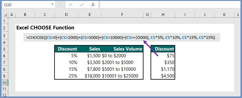
6. Calculate quantity discount with CHOOSE Function:
To calculate discount, we use the formula =CHOOSE((E6>0)+(E6>2000)+(E6>5000)+(E6>10000)+(E6>=25000), E6*5%, E6*10%, E6*15%, E6*25%), which returns the discount amount.
7. Use CHOOSE Function to return next working day:
To find the next working day in excel, the formula is =TODAY()+CHOOSE(WEEKDAY(TODAY()),1,1,1,1,1,3,2), which returns the next working day, assuming that today is SUNDAY. If today is Friday, use the reference 3.

8. Use CHOOSE Function with VLOOKUP:
To see the goals of a particular player, we use the formula =VLOOKUP(G5,CHOOSE({1,2}, D6:D10, C6:C10), 2, FALSE), which returns the number of goals of the particular player. If we change the name of the player, it returns the goals scored by the player.

9. Use CHOOSE Function to create Dynamic Chart:
To make a dynamic chart, we can use CHOOSE Function. Just the follow the steps below:
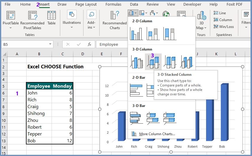
Step 1: Take the table with data from which you want to create dynamic chart:

Step 2: Select First and Second column and paste them into a new worksheet. Then select the columns (in our example B and C)–> Click on Insert –>click on second option of 3-D Column.
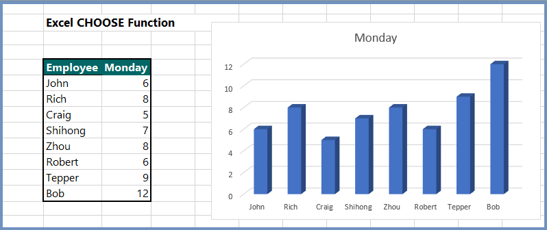
Now you have the following worksheet with the chart:
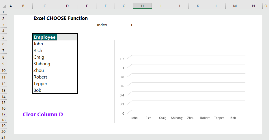
Step 3: Clear the column D, Monday. After clearing the column D, you see the following blank chart.
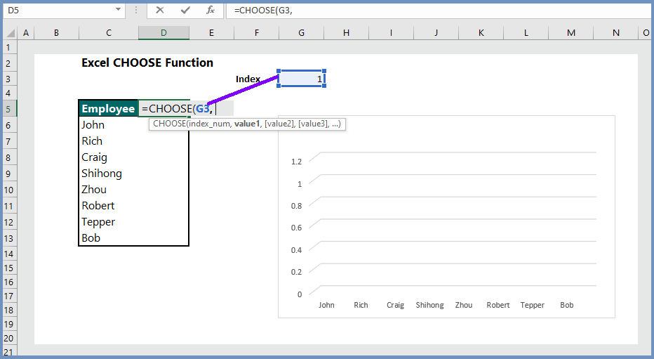
Step 4: Write the CHOOSE Function:
Write the CHOOSE Function in cell D5 as follows:
Start the formula
=CHOOSE(G3 //This is the index_num reference//
Add values:
Our values are located in the other worksheet (employee-work). Let’s jump across the employee-work data sheet and select the different days as follows:
=CHOOSE($G$3, ’employee-work’!D4,’employee-work’!E4,’employee-work’!F4,’employee-work’!G4,’employee-work’!H4) //

Now, pull down down the small square in fill the data.

Step 5: Insert Form Control:
To insert the Form Control, click Developer–> Insert –> Option Button.

Assign Index Number to Form Control:

You are done!!! Now change the index number and see the magic.
More readings:
1. CHOOSE Function MS Office Post
2. COUNTIF Function
3. AVERAGE Function
Thanks for sharing excellent informations. Your web-site is so cool. I’m impressed by the details that you have on this blog. It reveals how nicely you perceive this subject. Bookmarked this website page, will come back for more articles. You, my pal, ROCK! I found just the info I already searched all over the place and simply could not come across. What a perfect site.